Chapter 3 Getting started
We will use RStudio as a global interface to R. We’ll write code, open and save files, create and visualize plots, keep track of variables and R objects all within the same RStudio window.
In this chapter:
- Launching Rstudio
- Organize with an Rstudio Project
- Create an
Rscript - Working directory
3.1 Launch RStudio
TASK: Launch RStudio
To get started launch RStudio on your computer and it will access R automatically.
Both R and RStudio should be installed prior to class (see section 1.1.)
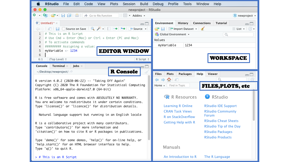
RStudio will open with 3 sections (called panes) if it is the first time you are using it:
- the R Console (left),
- Workspace area with Environment/History (top-right), and
- Files/Plots/Packages/Help/Viewer (bottom-right).
When we invoke the Source text editor it will automatically show at the top of the R Console on the left (see figure 3.1.)

Figure 3.1: The 4 quadrants of RStudio interface.
Note: the relative position and content of each pane can be customized with the menu cascade:
Tools -> Global Options -> Pane Layout
3.2 Organize with an RStudio project
It is a good habit to immediately create a project for handling the analysis of new data and keep everything together. RStudio can create the project directory if it does not exist, or it can use a directory that has already been set-up.
Having a single top-level directory to move the project to a different drive or into another directory, or to share it with collaborators. Subdirectories can also be used to better separate various files and data.
TASK: Create an R project
Start with menu cascade:File > New Project and then choose:
- New Directory
- Empty Project
- Chose a name for the directory, for example
learn-R - Keep the suggestion to create the project in
~/Desktop - Click on Create Project
From there it would be possible to create sub-directories from within the RStudio interface under the Files tab in the bottom-right pane. Alternatively the sub-directories could also be created from the familiar computer operating system interface.
For more complex project it may be useful to create sub-directories to contain data, scripts and other documents separately. For very complex data more sub-directories could be added such as an output directory for example.
For now we’ll just keep things under the same project folder.
3.3 Creating an R script
To more easily keep a record we’ll create a new text file with the built-in Editor.
TASK: Create script file
Use the following menu cascade to create a new script:
File > New File > R Script
You should now have a blank space on the left hand side as in figure 3.1.
This is where we’ll write R code and the file can then be saved to a plain text file that can be used again later. When saved the file will have a .R filename extension.
3.3.1 Script Editor
The editor is a plain text editor (no bolds or italics) but it offers color-coding of the text depending on what is written (syntax highlighting.)
3.3.2 Comments
While the code we write always makes sense right now it may not be obvious to others, including ourselves in the future. It is therefore extremely useful to comment the script with information such as giving a tile to sections or plain comments on the goal we are trying to accomplish.
Commenting is accomplished easily: each line with a a hashtag (#) is a comment and is ignored by R.
For example:
# This is a comment line
# I can write many comments to make sure I remember what I am doing
# The dir() function lists the content of the current directory
dir()  # comments can even be added here
Figure 3.2: Adding comments to scripts makes them easier to share with others, or your future self.
3.3.3 Executing commands
Commands that are written within the script can be executed by using the Ctrl + Enter shortcut (on Macs, Cmd + Enter will also work.) This will execute the command on the current line (indicated by the cursor) or all of the commands in the currently selected text.
This action will send the selected text to the R console that will run the commands. It is therefore the same as a Copy/Paste action from the script to the console, but easier.
3.4 Working directory
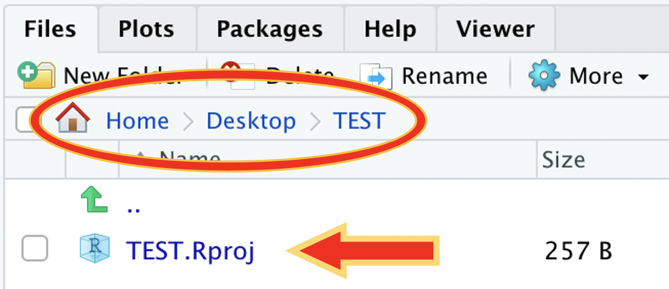
We created a new RStudio project earlier and the Files Tab on the bottom right pane shows the location of files and the “path” to this directory (red circle in figure 3.3.) It is possible to navigate the whole hard drive by using the 2 dots .. next to the “up” green arrow.

Figure 3.3: Files Tab shows files and path.
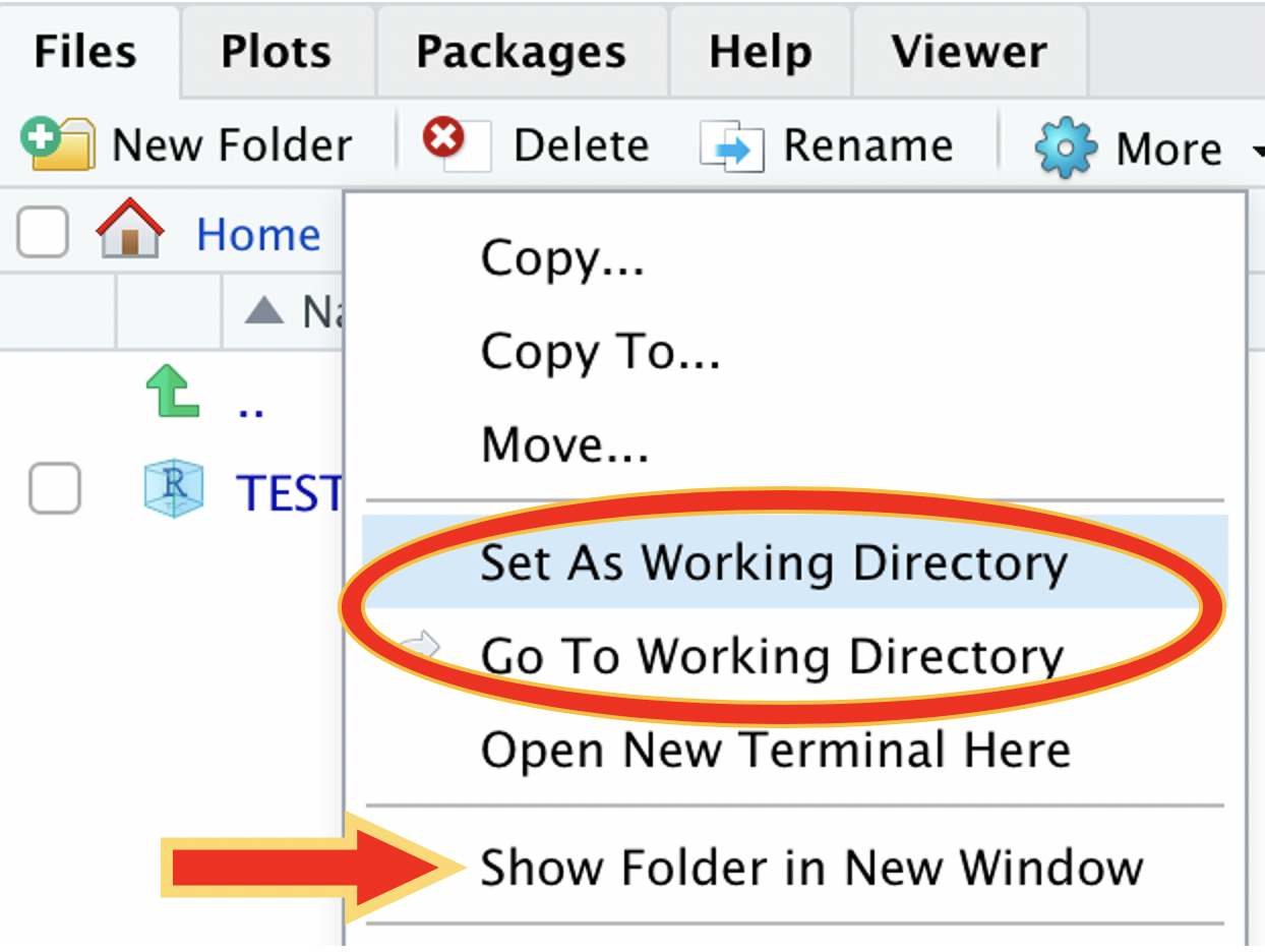
The More pull-down (3.4) menu makes it easy to return to the working directory if we got lost navigating the hard drive directory, to choose a new directory, or even to open the working directory on the computer graphical interface

Figure 3.4: More menu provides easy navigation to working directory.
In a section 4.3 we’ll learn command functions that can let us find or change the working directory from the R console.
